Do you want to know how to value growth companies?
Fundamentals 22. Growth is one of the key inputs when valuing companies. This post looks at the various issues to consider when valuing growth companies. Revision date: 14 Jan 2024
One of the challenges in valuation is how to bring growth into the picture. This will vary depending on your financial model.
- If you have a detailed financial model, you could have different growth rates for revenue and earnings.
- But if you are using a simple single-stage valuation model, what do you use to represent growth? Do you use the growth in revenue or the growth in earnings? They are not necessarily the same.
- And if you are using a multi-stage valuation model, there is the question of the terminal value. What should you use for the terminal growth rate?
The above is just one aspect of the issue. The more important one is how do you ensure that the growth rates you use are realistic? Then there is the issue of organic growth vs growth via acquisitions. Do you need to distinguish them?
In the context of fundamental analysis, growth is more than just looking at changes in a parameter. Digging into the drivers of growth can also provide insights that can help you formulate your investment thesis.
Join me as I illustrate the various growth issues based on some companies covered in my blog. Should go and buy them? Well, read my Disclaimer!
Note: This is an updated article that pulls together the following articles in my blog.
- Focusing on the assumptions of perpetual growth model.
- How to value high growth companies.
If you are tried to access the above 2 articles, you would be redirected here.
Contents
- Life cycle
- Valuation models
- DCF models
- Greenwald approach
- Estimating growth
- Estimating WACC
- Single-stage valuation examples
- 2-stage valuation examples
- Multi-growth valuation example
- Greenwald return example
- Conclusion
|
Life cycle
All businesses go through several stages in their corporate life. Damodaran has one framework for this as illustrated in Chart 1.
 |
| Chart 1: Corporate life cycle Source: Damodaran |
In his corporate life cycle model, there are 6 stages from Start-up to Decline.
In this model, growth companies are those that have gone beyond the Start-up stage but have yet to reach the Mature stage. It is relatively easier to identify the Mature stage. This is one where the growth rate is at best the GDP growth rate.
In real life, some established companies continue to deliver high growth rates. In the Damodaran corporate life cycle framework, you would classify them as being in the Mature-Growth stage.
To value a company from the Start-up to Decline stages, you need to capture the free cash flow at every stage. At the same time, you need different discount rates for each stage. This is because the discount rate is also intended to reflect the risk of the cash flow. This will differ for different stages of the life cycle.
It would be very challenging to project the cash flows and discount rates over the life of the company.
In practice, I seldom need to do this. I don't invest in Start-ups and Young Growth companies. This is because I don't know how to project their cash flows. As such, I focus on the High Growth, Mature Growth, and Mature Stable ones.
|
What to look for when valuing growth companies
The challenge for valuing companies at the growth stage is projecting the duration and the growth rates. Damodaran suggests that you need a narrative to help you do this. He then uses a DCF valuation approach to value such companies.
Bruce Greenwald believes that this sustainable growth characteristic is only applicable to "franchises". These are companies with some economic moat that enables them to sustain high growth rates.
He suggests an Asset Value vs Earnings Power Value comparison (AV-EPV comparison) to identify them. High-growth companies are those where the EPV far exceeds the Asset Value. He then verifies them by looking at their economic moats or competitive advantages.
According to Greenwald, the high growth duration depends on the strength of the moat. One way to gauge this is to see how long it would take for the competitive advantage to compete away.
If a company has moats that can provide "protection" for more than 2 or 3 decades, then it makes sense to determine the value of growth.
However, Greenwald believes that there are too many uncertainties when using a DCF model. Instead, he suggests that you look at the return space rather than the value space when figuring out the margin of safety.
|
Valuation models
The intrinsic value of a company is the present value of the cash flow generated by a company over its life. You first need to determine the cash flows.
Then to determine the present value of the cash flows, you have to discount them using different discount rates for each stage of the life cycle. This is because the discount rate not only reflects the time value of money but also the risk associated with the cash flow. The risks would be different for different stages.
The cash flows in turn depend on the growth pattern. There are 3 ways to incorporate growth into the cash flows according to the 3 common DCF valuation models.
You will notice that the 3 models assume that the company does not go into the Decline stage. If you accept the corporate life cycle concept, it must mean that the values determined by my valuation model are on the high side as it ignores the Decline stage.
Single-stage model
This is generally applicable to companies in the Mature Stable stage. At this stage, growth is assumed to be some low and steady rate.
I generally use this model for established brick-and-mortar companies that are not facing any disruption to their business. Examples of such companies include those in the steel sector, home builders, and household products.
I am not saying that there is no product obsolescence. Rather I am assuming that such companies will continue to develop new products to replace the obsolete ones.
You can understand my concern with using this model to value tech companies where the threat of decline is common. Think of Yahoo, Nokia, and BlackBerry and you will understand what I mean.
2-stage model
This divides the company's future cash flows into two distinct stages, each characterized by different growth rates as illustrated by the top picture in Chart 2.
 |
| Chart 2: Growth models |
The two stages typically include:
- A high growth stage. Here the company is assumed to experience rapid growth that may last for a certain number of years.
- A stable growth stage. After the high growth stage, the company is assumed to transition to a more stable and mature phase. It is often assumed to be in perpetuity and lower than the long-term GDP growth rate
I use this model for companies going through distinct growth phases. A good example of this is companies going through a high growth phase due to acquisitions before settling down to lower organic growth.
H-model or variable-growth model
There is also another model known as the H model where the growth rate drops gradually over time. Refer to the bottom image in Chart 1. This is often referred to as a "fade" in the growth rate.
The fading high growth rate is to reflect that a company's growth may be unsustainable at the initial high levels. And is likely to slow down as it matures or faces increased competition
There are standard formulae to determine the intrinsic values for these models.
In the past, it was difficult to calculate the intrinsic values for other growth patterns. But with EXCEL, this is not an issue anymore.
It is a simple matter to develop a variable growth model. In my DCF examples, I have different growth patterns for revenue, margins, and capital efficiency. I then computed the present values of the FCFF from the first principles.
DCF models
When you look at discounted cash flow (DCF) models, you either look at the cash flow to the firm or the equity holders.
I prefer to look at the firm model. There are a few key ideas behind this approach:
- Discounting to account for both the time value of money and risk.
- Using FCFF as the cash flow.
- Differentiating between operating and non-operating assets.
- The value of the firm accrues to all providers of capital.
There are 3 valuation gurus that I follow:
- Discounted Free Cash Flow to the Firm (FCFF) model as per Damodaran.
- Discounted Residual Income model as per Penman.
- Greenwald return method.
Each will have its strengths and issues. If your assumptions are consistent, both the FCFF and RI valuation models will give you the same answer.
In practice, the model I used for a company depends on the information available. I prefer the Residual Income model as it breaks down the firm value into 2 components. The first component is due to the Book Value while the other is due to excess earnings.
FCFF model
For the single-stage discounted FCFF valuation model, the value can be represented by the equation:
Value = FCFF × (1+g) / (r-g).
Where:
FCFF = the Free Cash Flow to the Firm
g = steady growth rate.
r = Discount rate = WACC.
It is referred to as the single-stage model because there is only one growth rate and one discount rate. It assumes that the FCFF increases annually by the same "g". It also assumes that the discount rate for the various periods is multiples of the same base WACC.
Note that the above model is a formula derived from the following present value equation.
You can see that it assumes the same growth rate and discount rate for all the years. It also assumes that the growth rate is an annual one. In other words, it increases once a year.
More importantly, the model assumes that the base year FCFF together with the growth rate is a good representation of the future cash flows.
Because of this, I spend considerable effort establishing the base FCFF. Sometimes I use the latest value. Sometimes I use the normalized value.
The FCFF can be thought of as the after-tax cash flow available to the providers of capital after accounting for CAPEX and increases in working capital. This is similar to what Warren Buffet calls "owners’ earnings". The "owners" here refer to all the providers of funds used by the company.
In practice, this FCFF is derived by first determining the earnings before interest and taxes (EBIT). You then act as if you paid taxes on the EBIT even though in real life, companies pay taxes after deducting interest charges.
You thus get the amount EBIT × (1-t) that is commonly written as EBIT(1-t) where "t" represents the tax rate. You next deduct any CAPEX and increases in Working Capital and add back Depreciation & Amortization.
Mathematically the FCFF can be represented by:
FCFF = EBIT(1-t) × (1-Re).
Where:
EBIT = earnings before interest and taxes.
t = tax rate.
Re = Reinvestment rate.
In principle, you can also determine the FCFF by deducting the Reinvestment items from EBIT(1-t).
I have carried out valuations where I first determined the actual FCFF for every year. I then determined the base FCFF as the average FCFF of the various years.
You should not be surprised that the base FCFF derived from this average method is different from that derived based on EBIT(1-t) x (1-Re).
Which is more appropriate? I don't think there is an answer. Each is based on a different set of assumptions.
I prefer to use the one based on EBIT(1-t) × (1-Re) because I can link the growth rate to EBIT. If I use the average FCFF approach, I would have to link the growth rate to the growth in the FCFF.
Residual Income Model
In the Residual Income approach, the intrinsic value of the firm is the Total Capital Employed (TCE) plus the present value of the Residual Income.
Residual Income (RI) is defined as the after-tax EBIT minus a Capital charge. The relevant cash flow here is the Residual Income.
TCE = Shareholders Funds + Minority Interests + Debt - Cash & Other Non-operating Assets.
For consistency, the TCE should be the capital employed to generate the EBIT.
The Capital charge is represented by WACC × TCE.
RI = EBIT(1-t) - (WACC x TCE).
Both the FCFF and RI models value the operating assets. To determine the value of the firm, you have to add the value of the non-operating assets.
My valuation models focus on the value of the firm. To determine the value to equity holders, I then deduct the value of debt and minority interests.
Operating and non-operating assets
EBIT is generated by the operating assets.
Examples of operating assets are plant & machinery and net working capital. It excludes cash, investment in associates, and investment in securities as these are generally not considered part of the normal business operations.
Given this, the intrinsic value of the firm = Value of operating assets + Value of non-operating assets.
In other words, you have to add the value of cash and other non-operating assets to the value obtained from discounting the FCFF.
This would require you to determine the values of the various non-operating assets. For example, for investments in other companies, you should use the appropriate portion of the intrinsic values of these companies.
In practice, I take cash and other non-operating assets at their Book Values. I assumed that they are small components of the total intrinsic value. Determining the intrinsic value of these non-operating assets would not make a big difference to the total intrinsic value.
Value to all providers of capital.
In both the FCFF and RI model, the value obtained by adding the operating assets and non-operating assets belongs to all the providers of funds.
To determine the value to the equity holders you have to deduct what is due to the other providers of funds. These are the portion due to the minority shareholders and those providing Debt.
Technically Debt should be based on the market value of Debt rather than the Book Value. There are theoretical ways to determine the market value of Debt but this is a story for another day. In practice, if the amount is small eg DE ratio is less than 1, I assumed the Book Value.
Similarly, I also use the Book Value when considering the value of the Minority Interests.
You can see that assumptions are made from the start - the stages of the life cycle, Value of non-operating assets, Value of Debt, and Value of Minority Interests. This is even before considering parameters used to determine the value of the operating assets.
|
Greenwald Return approach
There are 3 steps in Greenwald approach:
- Using the AV-EPV comparison to identify the high-growth companies.
- Verifying then with competitive analysis.
- Determining the Returns.
According to Greenwald, EPV > AV can only be sustainable if there is some moat. You verify this via a competitive analysis.
As for the Returns, Greenwald classifies them into 3:
- Cash returns. These are from Dividends and buybacks.
- Returns from reinvestments. For this to have value, the return has to be greater than the cost of capital.
- Organic growth This comes from the general economic growth and Greenwood considers them as "free".
Greenwald formula contains 3 components. The first component is for the cash returns. The second component refers to the returns from reinvestments. The last is for organic growth.
Expected return = b(E/P) + (1-b)(E/P)(ROE/r) + g
Where:
b = portion of earnings distributed.
E = Earnings per share.
P = Price per share.
ROE = Return on Equity
r = Cost of Equity.
g = growth.
Based on the historical data, you determined the amount set aside for Dividends and share buybacks.
You then estimate the Return from this component by dividing it by the EPS. This is your first Return component. Let us assume that this is Y %.
You next estimate what is available for Reinvestment by deducting the portion for Dividends and share buybacks. You then determine the reinvested Return. This is not merely dividing by the EPS. Let us assume that the return with this simple division is Z %.
Rather he estimates whether the reinvested Return would be higher or lower than Z %. He does this by comparing the marginal return on capital with the marginal cost of capital.
For example, if the return is 15% compared to the 10% cost of capital, it means that for every dollar invested, the company gets 1.5 dollars of return. He then assumed the reinvested Return to be 1.5Z %.
From what I could see, Greenwald considers that there is no need for any investment to generate organic growth.
However, instead of using the long-term GDP growth rate as the organic return, he makes certain adjustments.
- He adds 1% if the company serves the luxury market.
- He deducts 3% if the company serves the mass market.
- He deducts 0.5 % if it sells goods rather than services.
In his example, the long-term US GDP growth rate of 4 % translates to 0.05 % organic Return after the above deductions.
We now have the 3 components to estimate the total Return = cash Return + reinvested Return + organic growth.
In our example, this = (Y + 1.5Z + 0.05) %.
Greenwald then compares this with the cost of capital to look for the margin of safety.
The amount of margin of safety should be linked to the strength of the moat. If you have a moat that takes a decade to be eroded, you want a higher margin than one with 5 decades of protection.
Limitations of the Return Approach
According to Greenwald, the main problem with the Return approach is that there is no dollar estimate of the intrinsic value. As such it is more difficult to determine when it is overvalued.
According to Greenwald, investors such as Warren Buffet and Seth Klarman set some guidelines. Warren Buffet supposedly holds the stocks forever. Seth Klarman has some PE cut-offs.
I would have thought that a reasonable sell guideline would be when the total Return is half of the cost of capital. Unfortunately, I do not have sufficient such types of investments to see whether this guideline is workable.
Organic Return
There are 2 issues here:
- What is the organic return?
- What is the Reinvestment required for the organic return?
I have discussed how Greenwald treated the organic return as one with zero reinvestment. But then he adjusts the long-term GDP growth rate to derive the organic growth rate.
I have seen a Greenwald article where he used the long-term growth rates in productivity and profit margin as the free organic return.
The logic of the free organic return can be seen from the dividend discount model.
P = D/(r - g).
Return = D/P + g.
However, I saw an article where some reinvestment was deducted to get the return from organic growth.
If you look at the Greenwald return formula, you can see that the organic growth rate can have a significant impact on the total return. As such I would take a conservative estimate and not use the full GDP growth rate.
Damodaran has suggested that the long-term growth rate for the terminal value be set at the risk-free rate. I think this is a good rate.
The best way is to think of the growth that can be achieved without any investment. Examples are:
- If you are a retailer, this could be same-store sales.
- Improvement in operating margins by being more efficient.
- Changes to higher margin product mix to get better margins.
Estimating growth
The growth rate you choose will significantly impact the valuation of the company. Here are some key steps and factors to consider:
Historical Growth. I look at the company's historical revenue growth rates to identify trends.
Industry Benchmarks. For high-growth situations, I also consider the overall growth prospects of the industry and whether the company is expected to outperform or underperform its peers.
Management guidance. Some analysts rely on the company's management regarding future growth prospects. This can include official guidance, earnings calls, or analyst presentations.
Market research. I also look at industry reports and growth projected by market research houses.
Insights from Reinvestments
Reinvestments can also provide insights into the long-term growth rate. The underlying assumption here is that the long-term growth rate will be less than the discount rate. Next, growth is assumed to be the same in perpetuity.
For this to be realistic, the growth rate has to be smaller than the GDP growth rate. Damodaran has even suggested that it should be the risk-free rate.
Growth in this context comes from the fundamental growth equation where:
Growth = Return X Reinvestment rate.
In the context of the firm,
Return = EBIT(1 – t) / Total Capital Employed
t = tax rate
Total Capital Employed = Equity + Debt – Cash
Reinvestment = CAPEX + Acquisitions – Depreciation & Amortization + Net Changes in Working Capital
Reinvestment rate = Reinvestment / EBIT(1-t)
In using the fundamental growth equation, you need to ensure that you are consistent. If growth is based on Total Assets, then the return should be based on Total Assets. If growth is based on the Total Capital Employed, the return should be based on the same metric.
Even when using the fundamental growth equation, you have to check that the growth is realistic. This is because growth is dependent on the Reinvestment rate and Return. You have to check that what you assumed for these is realistic.
There are a few ways to carry out such a sanity check. Look at the historical performance. Look at industry performance. I also look at market research reports to get a sense of the revenue growth rate. And don’t forget to cap the terminal growth at the long-term GDP growth rate.
Estimating the TCE
The challenge here is determining the TCE. To estimate the TCE, I first determine the average TCE/Revenue ratio for the company.
With this ratio, I then determine the TCE for the projected Revenue. We can then use this to derive the corresponding Return. Thereafter we can derive the Reinvestment rate.
The key assumption here is that the Reinvestment rate is constant. In many cases, you will find that the actual historical Reinvestment rate differs from the derived rate.
This is partly because CAPEX is a lumpy expenditure in real life. Secondly, management has some discretion in managing working capital.
The other assumption is that there is some fixed ratio between TCE and Revenue.
The TCE/Revenue ratio is similar to the inverse of the Asset Turnover. In the DuPont analysis, there is a link between the ROE and Asset Turnover. We can imagine a similar relationship between the Return defined here and the TCE turnover.
If we assume that the Return is stable, then the TCE/Revenue ratio should also be stable.
Estimating WACC
Because I am looking at the cash flows to the firm, the discount rate used is that for the firm. This is commonly called the weighted average cost of capital (WACC) as it takes into account the cost of equity as well as the cost of Debt.
The cost of equity is derived from the Capital Asset Pricing Model (CAPM). This requires assumptions about the risk-free rate, the risk premium, and the risk.
Risk in this context is measured by the Beta of the firm. In other words, you assumed that volatility = risk.
The cost of Debt is based on viewing all the Debt as equal to a single bond. It is not the Book Value of Debt.
According to Investopedia, one way to calculate the after-tax cost of Debt = (risk-free rate + credit spread) × (1-t).
You will appreciate that there are assumptions to derive the cost of Debt. Damodaran has a good write-up on the WACC. Refer to “The weighted average cost of capital – NYU Stern”
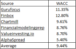
In practice, I sometimes derive the WACC following Damodaran's approach. But for US companies there is a lot of readily available information. As such I used the average value based on a Google search of the WACC.
A good example is how I derived the WACC for the building materials distributor BlueLinx as shown in Table 1.
The key point is that there are several assumptions in estimating the WACC. As such, there is no one figure for the WACC.
 |
| Table 1: Estimating the WACC for BlueLinx |
Single-stage valuation examples
For this example, I used the valuation of Tempur-Sealy, a US bedding company as shown in Table 2. For details refer to “Tempur Sealy Is A Cyclical Company And Should Be Valued As Such”
 |
| Table 2: Estimating the Value of Tempur-Sealy |
Table 2 illustrates how I computed the intrinsic value based on the single-stage discounted FCFF. It takes into account the value of the operating and non-operating assets. It deducts Debt and minority interests to get to the value to the equity holders.
I determined the value of the operating assets as UDS 6,852 million - item “p” in Table 2.
I then added the non-operating assets – item “s” in Table 2.
But I have seen arguments that if companies have a bad track record in deploying cash, there should be a discount to the Book Value. This is especially true if the cash component is significant.
EBIT
The starting point in my valuation model is how I derive the FCFF. This in turn depends on how I derive the EBIT.
The assumptions used to derive the EBIT are generally tied to the company's characteristics. This will differ from case to case. As such I will just cover the general assumptions here.
There are several ways to derive the EBIT. In the model shown in Table 2, the EBIT was derived based on Gross Profit less SGA expenses. Refer to item “f” in Table 2.
Gross Profit = Revenue × Gross Profit margin.
SGA = Revenue × SGA margin.
The Revenue, Gross Profit margin, and SGA margin are "normalized" values. How I derived the "normalized" values would depend on the company. In the Tempur-Sealy case as per Table 2, the normalized values were based on:
- The current revenue. This is to reflect the current size of the company.
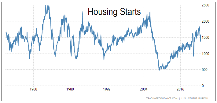
- The normalized gross profit margins and SGA margins. These were based on the values over the cycle. The cycle period was assumed to be from 2014 to 2022 based on the Housing Starts cycle.
In the case of Housing Starts, the actual peak-to-peak was 2005 to 2022 as shown in Chart 3. But unfortunately, Tempur-Sealy in its current form came into the picture in 2013. Thus, the only data available for determining the average values was from 2014 to 2022. The assumption is that this period is a good representation of the cycle.
 |
| Chart 3: US Housing Starts. Source: Trading Economics.com |
As can be seen, the starting point for my valuation was Revenue. The value for this metric will depend on the situation.
In my Steel Dynamics analysis, I determined Revenue by looking at the shipping tonnage and then relating this to the long-term average revenue per ton. Steel is a cyclical commodity and while unit prices vary widely throughout the cycle, the shipment quantity is more "stable". Growth came from the shipment tonnage rather than the cyclical prices.
In my Boise Cascade analysis, I pegged Revenue to the long-term average annual Housing Starts. This is because while House Starts are cyclical, there is no growth in the long-term average annual Housing Starts of about 1.5 million units. The Revenue is for the year when the Housing Starts was 1.5 million units.
The underlying assumption here is that the margins are stable within the range of Revenue considered. We know that certain items in the cost of sales eg depreciation and staff costs do not vary per unit of output. Rather they have stepped changes. But we act like they are continuous variables. This is a reasonable assumption if the volume is far above the breakeven level.
Tax rate
According to Damodaran, we should use the nominal tax rate rather than some average of the actual tax rate. This is because we are taking a long-term view whereas actual tax rates may be affected by short-term tax adjustments.
Using a nominal rate works if the company operates in only one country. However if the company operates in several countries with different tax codes, I find it difficult to determine a nominal rate. In such cases, I used the actual average tax rate.
In practice, changes in the tax rate are not as significant as changes in the FCFF or WACC on the intrinsic value.
SGA
Selling, general, and administrative expenses generally have step changes. Even if you consider them variable, they should only apply to a particular Revenue range.
In the example shown in Table 2, I have assumed that the SGA is a variable linked to the Revenue. That is why I used the SGA margin.
Alternative EBIT approaches
The model illustrated in Table 2 is not the only way to determine the base year EBIT or normalized EBIT. The template shown is a general one. But there are other ways involving different assumptions as illustrated by the following.
In my Leggett & Platt analysis, the EBIT was based on the EBIT/Total Asset ratio. The growth was then the growth in Total Assets. This was because it was difficult to estimate the Gross Profit margin or SGA margin. Refer to “Leggett & Platt: Limited Financial Benefits From ECS Acquisition”
In the case of Stelco, I used the average EBITDA and then deduct Depreciation & Amortization to derive the EBIT. In that case study, there was not enough information to derive the Gross Profit margin. Refer to “Stelco Holdings: Grossly Underpriced Cyclical Growth Company”
In the Timken Steel analysis, I estimated the Gross Profit for the base year directly by taking the average Gross profit. I then deducted SGA to arrive at the EBIT. This was because the company was operating below breakeven levels for most of the period. For the base year, I wanted the intrinsic value if it operated above this breakeven level. Refer to “TimkenSteel: Under-Priced Even Through A Cyclical Lens”
2-stage valuation examples
Here, I would use CBIP to illustrate the valuation. Refer to the blog article for the details of the company.
I first invested in CBIP in 2017. I had considered this a compounder based on the following:
- From 2007 to 2016 revenue grew at 8.0 % CAGR and PAT at 10.2 % CAGR.
- ROE averaged 20.6 % from 2007 to 2016.
- Shareholders’ funds grew at 17. % CAGR from 2007 to 2016. This was mainly from retained earnings. While there were several rounds of bonus issues, there was no call for additional paid-up capital.
I would not go into the details on why I think CBIP is a good company here. Refer to my blog article if you want the details.
I use CBIP as the case study to illustrate the various computations. Table 3 summarizes the key parameters required for the valuations. They cover the key value drivers as per Damodaran.
- Revenue and the growth rates.
- Gross profit and SGA margins. I also assumed that these would change over time.
- Capital efficiency as measured by the TCE/Revenue and the growth rates.
- Some measures of how to fund the growth. I generally use the Reinvestment rates.
- The discount rates. I have derived the Cost of Equity and the WACC based on the Damodaran build-up method.
 |
| Table 3: CBIP Parameters |
For this case study, I will assume that there is some growth narrative that matches the numbers shown in Table 3. I will not cover the narrative but focus on the computation aspects.
I will illustrate how I determined the intrinsic value of CBIP using both the FCFF model as well as the Residual income model.
FCFF valuation
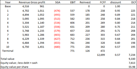
I used a 2-stage FCFF model to value CBIP where there is a high revenue growth stage followed by a lower long-term revenue growth rate.
Table 4 and the accompanying notes illustrate the computation.
I assumed that the high revenue growth stage to be 5 years. The model assumes that the low-growth stage continues in perpetuity. In other words, I do not factor in any decline.
I have also assumed growth for other parameters – margins and capital efficiency. If you look at columns b, c, and f for the various years, you can see the changes.
The key parameters for each stage are the FCFF and the WACC. The FCFF for each stage in turn depends on the EBIT, tax rate, and Reinvestment rate.
As in my earlier article, I assumed that growth is determined by fundamentals.
g = Return × Reinvestment rate.
Return = EBIT(1-t)/TCE. Note that I used the TCE of the previous period.
So if I can determine the TCE for each year I can then determine the Return for each year. Thereafter I can determine the Reinvestment rate for each year.
Conceptually I am determining the FCFF for each period and then discounting it to the present value ie year = 0.
The intrinsic value is the sum of all the individual discounted values. Note that the value of the mature stage is also discounted to the present value.
Based on this model, the intrinsic value of CBIP is RM 1.81 per share compared to the market price of RM 1.80 per share.
Residual Income valuation.
In this model, the key parameters for each year are the TCE and the WACC. This will enable us to determine the Residual Income for each year.
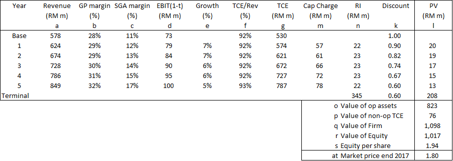
Table 5 illustrates the computation. I have assumed the same parameters for CBIP as those in the FCFF valuation example.
Based on the TCE/Revenue ratio, I then projected the TCE for each year. Given the WACC, I then determined the Capital charge for each year. Note that I used the TCE for the previous period to determine the current period Capital charge.
I then determined the Residual Income and the corresponding Terminal Residual Income. I determined the Terminal Residual Income using the perpetual growth formula.
The value of the operating assets to the Firm = current TCE + total present of the Residual Income.
Based on this model, the intrinsic value of CBIP is RM 1.94 per share compared to RM 1.81 per share from the FCFF model.
In theory, both approaches should give the same answer if the assumptions are consistent. The difference meant that I had some inconsistencies in my assumptions. In practice, I seldom get the same answers so I generally take the average of both models as the final intrinsic value.
 |
| Table 5: Residual Income Valuation of CBIP Refer to the Notes in Table 4 for the explanations of each of the alphabet notes. |
If I assumed that all the growths – revenue, margins, capital efficiency – are zero, we have the Earnings Power Value (EPV). This is RM 1.68 per share.
Multi-growth valuation example
For this example, I will use my analysis of Leggett & Platt, a US components company. Refer to the following for details:
LEG growth was via a combination of organic growth and non-organic growth. Growth via acquisitions is quite significant. From 2015 to 2022, revenue grew at a 4.2 % CAGR, while EBIT grew at 3.6 % CAGR.
To further confuse the matter, total assets grew at a CAGR of 10.1 %. The point is that there are many growth components.
Given that there were many different growth rates, the best way to model LEG is to develop a financial model with the various growth parameters.
The endpoint is to determine the Free Cash Flow to the Firm (FCFF) for various periods. The value of the firm is then the total discounted values of each period FCFF including the terminal value.
One format is shown in Table 6 where there are main two growth phases:
You can see from Table 6 that you could have different growth rates for the various parameters. In the example in Table 6, I assumed the following:
- 4.1 % annual growth for revenue.
- The gross profit margin improved by 1% every year.
- The SGA margin improved by 2% every year.
- A stable Reinvestment rate of 42.8 %.
- The terminal growth rate of 2 % in perpetuity.
- The same discount rate for all the years.
While theoretically correct, the above requires you to make assumptions about the various growth rates. The challenge is not the development of the financial model. It is whether the assumptions about the growth rates for the various parameters are realistic.
Greenwald return example
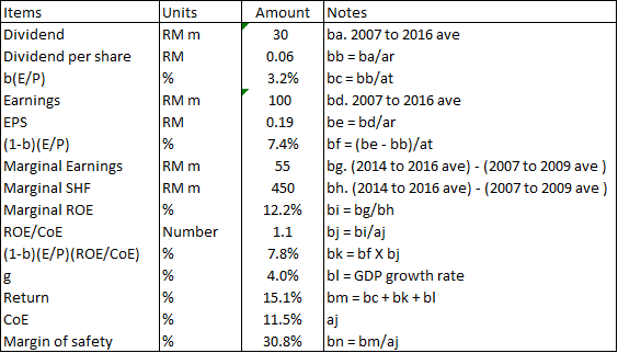
In this section, I illustrate how I used the Greenwald approach to determine the return for CBIP using the following formula.
Return = b(E/P) + (1-b)(E/P)(ROE/r) + g
Table 7 illustrates how I derived the values for each component.
Based on this approach, I estimated the total return = 15.1 %. If I compare this with the Cost of Equity of 11.5 %, there is a 30.8 % margin of safety.
On this basis, I concluded that there is a margin of safety. This was even though there is no margin of safety based on the DCF approach.
In my work example, I have assumed that organic growth is the GDP growth rate.
Conclusion
All valuations are based on assumptions. There are several types of assumptions involved:
- The valuation model used.
- The values of the non-operating assets.
- The values of Debt, Minority Interest, and other non-equity provider of funds.
- The values of the key parameters to determine the FCFF.
The point is that it is not just the assumptions to derive the FCFF. As shown in this article there are other assumptions. With so many assumptions you could be forgiven for doubting the accuracy of the value obtained.
I agree. That is why we have a margin of safety.
Given the many assumptions you may also wonder why to bother with the DCF method when relative valuation is much simpler. However, when you use relative valuation, you are pretending that there is no assumption. In reality, the assumptions are implicit.
With the single-stage discounted FCFF model, the assumptions are explicit and can be easily challenged. I rather know that they are based on assumptions than not knowing what has been assumed as with the relative valuation method.
In valuing companies, we make many choices and the intrinsic value obtained reflects the choices made. That is why different people will get different intrinsic values even though they all use the same single-stage discounted FCFF approach.
Damodaran and Greenwald have proposed different valuation approaches for high-growth companies.
- Damodaran approach with the narrative and FCFF model applies to companies coming out of the start-up stage. With these companies, there is hardly any operating history. At the same time, the lack of historical data may make AV-EPV comparison difficult.
- Greenwald approach is more suitable for established companies with growth rates far over the GDP growth rates. His AV-EPV comparison is a good starting point for identifying such high-growth companies. You then verify them by identifying the competitive advantages.
Note that in Greenwald’s approach, the high growth rate is not the main metric. Greenwald looks at the return space to determine the margin of safety.
I hope I have made a case for both to be in your valuation toolbox.
End
- - - - - - - - - - - - - - - - - - - - - - - - - - - - - - - - -
How to be an Authoritative Source, Share This Post
|
Disclaimer & Disclosure
I am not an investment adviser, security analyst, or stockbroker. The contents are meant for educational purposes and should not be taken as any recommendation to purchase or dispose of shares in the featured companies. Investments or strategies mentioned on this website may not be suitable for you and you should have your own independent decision regarding them.
The opinions expressed here are based on information I consider reliable but I do not warrant its completeness or accuracy and should not be relied on as such.
I may have equity interests in some of the companies featured.
This blog is reader-supported. When you buy through links in the post, the blog will earn a small commission. The payment comes from the retailer and not from you.





Comments
Post a Comment